How London Dispersion Forces Really Work:
Eighty-seven years later, Fritz London would like a word with us.
Losing the Plot
If London Dispersion Forces (LDF) worked the way that they are often taught, there would not be anyone around to actually teach them.*
It all starts out on the right track.
As noble gas atoms bounce around, electron clouds within them also bounce around, producing tiny, transient atomic dipoles. In the gelid conditions produced in cryopumps, these atoms listlessly approach each other and their tiny dipoles attractively align under the spell of a quantum mechanical incantation called electron correlation.
The atoms get sticky. And Nature says,
“Let there be liquid.” And there is liquid.
Suddenly, we understand LDFs!
We assume that LDFs work the same way in molecules as they do in noble gas atoms, which, as you will soon see, means that LDFs can be only INTER-molecular.
That brings us back to our *species’ hypothetical non-existence. Biological function of the proteins that animate our very existence depends on the tendency of these long-chain molecules to fold in three dimensions in extremely specific ways. As it turns out, at least 60% of protein folding stabilization is due to hydrophobic interactions – aka INTRA-molecular LDFs (Pace2014).
Well then, if the LDFs that we teach can be only INTER-molecular, somewhere along the way we have lost the plot.
“No problem,” you say. “I teach chemistry, not biochemistry. Protein folding is not on my syllabus. My LDFs only need to be able to explain the boiling points of small, nonpolar molecules.”
Not so fast.
As I will soon demonstrate, the LDFs that we currently teach do not even correctly explain the boiling points of the structural isomers of pentane.
Gaps
As of this year (2023), I have been building simulation models of the forces within and between atoms and molecules – including LDFs – for forty years. For the last decade or so, I have been adapting and developing these models to show students and teachers how atoms and molecules really work.
As I have observed how we teach chemistry, I have sometimes been struck by the large gaps between:
how we teach certain chemical phenomena
what we know about how they actually work – via theory, simulation, and experiment.
and
LDFs are one such phenomenon.
Some History
The earliest recorded contemplations of the interactions between molecules in the liquid (vs. the gaseous) state are credited to German physicist Rudolf Clausius in 1857. (Clausius1857) .
We have filled in a lot of the details since then.
In 1930, Fritz London, at the University of Berlin, published his quantum mechanical interpretation of van der Waals forces, including the attraction between noble gas atoms – what we now call London dispersion forces (London1930) . The first crude computer simulations of simple gases were carried out in the late 1950s (Alder1958) . The first full-scale simulation of a protein was performed in the late 1970s (McCammon1977) . And the impact of molecular simulation on our understanding of matter was recognized by the 2013 Nobel Prize in Chemistry.
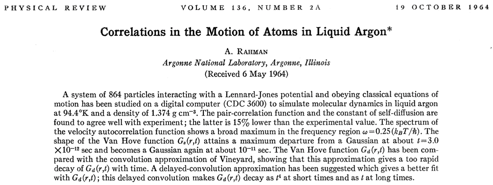
Figure 1. Publication of the first realistic simulation of LDFs in argon in 1964.
The first realistic computer simulation of LDFs of a substance in a condensed state was performed in 1964 (Fig. 1). Anees Rahman, of Argonne National Laboratory, performed a simulation of 864 liquid argon atoms. The potential energy of interaction between the atoms – due to LDFs – was modeled using the Lennard-Jones potential energy function (discussed below).
LDFs in Atoms
With their filled valence shells and no polar bonds to participate in dipole-dipole interactions, noble gases and nonpolar molecules should never stick together to form liquids or solids. So, why do they?
Via the magic of Atomsmith, let’s take a look: the negatively-charged electron clouds in noble gas atoms (helium in this case) are always oscillating around their positively charged nuclei. And as they vibrate, they form tiny, temporary dipole moments within each atom (Animation 1, below).
Under very cold conditions, as noble gas atoms approach each other, their tiny, temporary dipole moments align to produce an attractive interaction between them (Animation 2, above).
And now you may be wondering…
“Why do the atomic dipoles align when they get close? That seems counterintuitve. Shouldn’t the electrons repel each other when they get close?”
The dipole moments align due to electron correlation, which is a purely quantum mechanical effect – the difference between the exact non-relativistic solution of the Schrödinger equation, and the Hartree-Fock limit, within the Born-Oppenheimer approximation (Silva2020).
Aren’t you glad you asked?
The strength of this attractive LDF force between a pair of atoms, like the two helium atoms, is largely determined by two factors:
- magnitudes of the temporary atomic dipole moments
Larger dipole moments mean greater attractive (negative) LDF potential energy.
In turn, the dipole magnitude within each atom depends on two factors:
- atomic polarizability
Larger atoms (atoms with more volume) have more room for the electron clouds to “bounce around” – they are more polarizable, resulting in larger dipole moments.
- number of valence electrons
Valence (outer shell) electrons are held less tightly to the nucleus, so they contribute most of the motion that creates the temporary atomic dipole moments.
- atomic polarizability
- distance between the atoms/dipoles
When the atoms are very close to each other, their temporary dipole moments align and the dipole-dipole attraction is greater.
Let’s consider the LDF interactions in three noble gases: He, Ar, and Kr. The most commonly used LDF potential energy function is the Lennard-Jones potential. Fig. 2 (below) displays LDF potential energy vs. atom-atom distance for these three gases.
Eq. 1 (below) is the functional form of the Lennard-Jones potential, in which $r$ is the distance between the atoms. The first term (proportional to $r^{-12}$) corresponds to the repulsive (left-) side of the curve. The second term (proportional to $r^{-6}$) , corresponds to the attractive (right-) side of the curve.
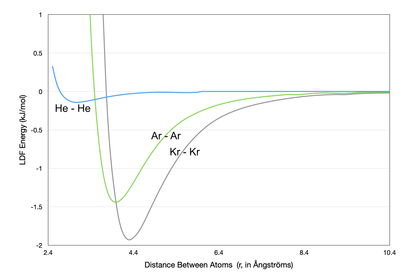
Figure 2. Lennard-Jones potential energy (ULJ) curves for He, Ar, and Kr.
$${U_{LJ}}=\frac {C_{12}} {r^{12}}-\frac {C_{6}} {r^{6}}$$
Equation 1. The Lennard-Jones (LJ) equation is used to model the LDF potential energy (ULJ, Fig. 2) due to the interaction between a pair of temporary atomic dipoles. $r$ is the distance between the two atoms. The $C_{12}$ constant determines the steepness of the repulsion (left side of the curve) for a pair of atoms. The $C_6$ constant determines the attractive potential energy well depth for a pair of atoms.
The depths of the three potential energy wells in Fig. 2 correspond to:
- the magnitudes of the dipole moments within the atoms and
- the boiling points
of each substance.
The ordering of the magnitudes of the atomic dipole moments (and corresponding boiling points) can be rationalized by using the explanation of LDF strengths from above:
- He atoms have the smallest polarizability (~volume) and only two valence electrons
- Ar atoms have a slightly larger polarizability (~volume) and eight valence electrons
- Kr atoms have the largest polarizability (~volume) and eight valence electrons
This same logic – comparing the numbers of valence electrons and the atomic polarizabilities (~volumes) – can be applied to estimate the strength of the LDF interaction between any pair of atoms, intra- or inter-molecular.
Note: Remember the $r^{-6}$ dependence of the attractive term in the Lennard-Jones potential. This is the term responsible for the short-ranged nature of LDF interactions. It will play a role in the Misconceptions section below.
LDFs in Molecules
Now that we have explained how LDFs work in atoms, let’s turn to how they work in molecules.
Here is what is different:
NOTHING! (Well, almost nothing.)
Everything that we said about LDFs in atoms applies equally to LDFs in molecules.
But you need to realize that, unlike in metals, the electrons in covalently bonded molecules generally don’t just “flow” between atoms. So the dipoles that cause LDFs in molecules are within each atom – just as they are in noble gases.
The total LDF potential energy in a system of molecules is simply the sum of all atomic dipole - atomic dipole interactions across all molecules in the system (Figs. 3 and 4).
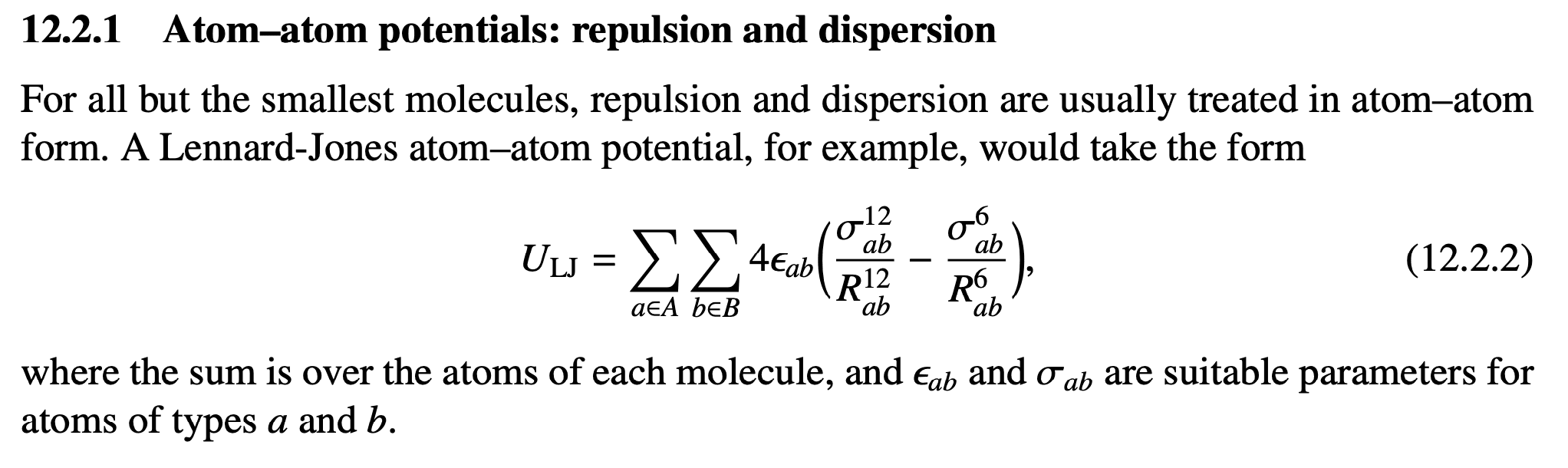
Figure 3. Since the time of Rahman’s simulation of argon atoms in 1964, we have understood that LDF interactions are atom-to-atom interactions. The statement above by Anthony Stone of Cambridge University – one of the foremost experts on the theory of intermolecular forces – summarizes this idea.(Stone2013)
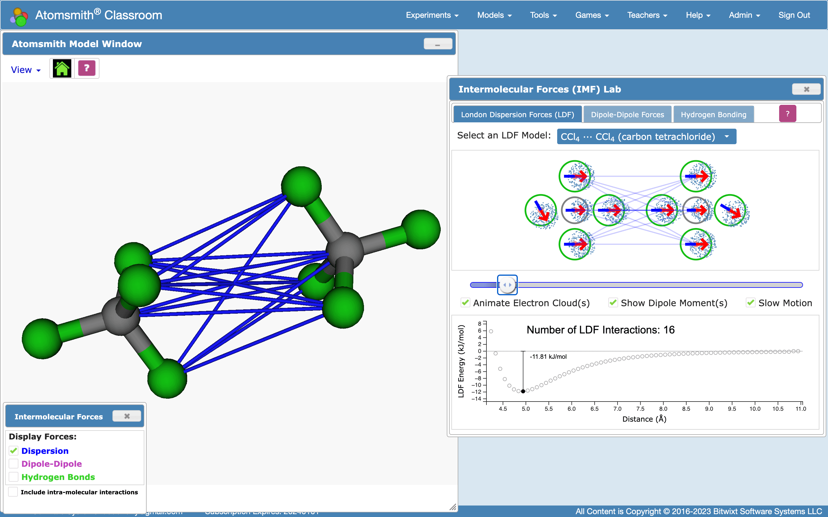
Figure 4. Two carbon tetrachloride (CCl4) molecules interacting in the Atomsmith Intermolecular Forces Lab, via their aligned, temporary atomic dipoles (right). Notice that some atoms in these two molecules do not participate in LDF interactions (displayed as thin blue lines).
LDFs are a universal force – they are present in all of the following:
atoms, polar molecules, nonpolar molecules, and even ions.
When applying LDFs to nonpolar molecules – molecules for which they are the only IMF present – there are two primary cases:
- Molecules with the same structure and different substituents
Consider the series of molecules: CH4, CF4, and CCl4 (see Fig. 4, above). They all have the same bonding structure. Therefore, as pairs of each of these molecules approach each other, they exhibit the same atomic dipole - atomic dipole interactions.
To explain the differences in LDF energies (and corresponding boiling points) in these molecules, one should recognize that the numbers of atom - atom LDF interactions between pairs of molecules are the same. Therefore, the only way to explain the differences in LDF energies (and corresponding boiling points), is to use the differences in atomic polarizabilities (~volumes) and numbers of valence electrons of the different substituents (e.g., H, F, or Cl) – just as described above for the series of noble gas atoms.
- Molecules with the same substituents and different structure
Here, one can use Atomsmith to investigate molecules that contain the same substituents, but have different 3D structures – for example, different structural isomers of the same alkane, such as n-pentane and neopentane. In this case, the difference in LDF energies (and corresponding boiling points) is due to different numbers of LDF atom - atom interactions, because of differences in shape.
The Bottom Line
To understand LDFs in molecules, you simply need to answer these two questions about the atom - atom LDF interactions:
- How many atom - atom interactions are there?
This is determined by the shapes of the molecules.
- How strong is each type of atom - atom interaction?
This is determined by the types of atoms in the molecules.
Next, read on if you want to dig into more detail and to contrast this model with how LDFs are widely taught.
Misconceptions
(Here be Dragons)
How LDFs Really Work
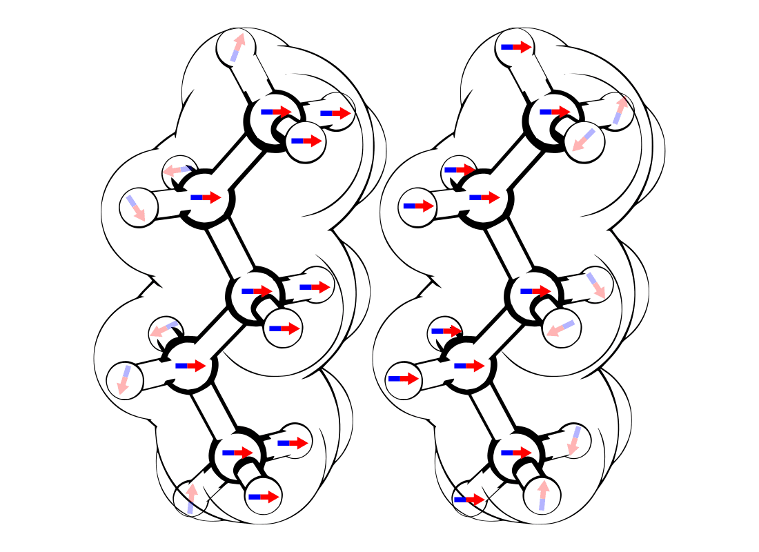
Figure 5. LDFs as atomic dipoles.
How LDFs Are Taught
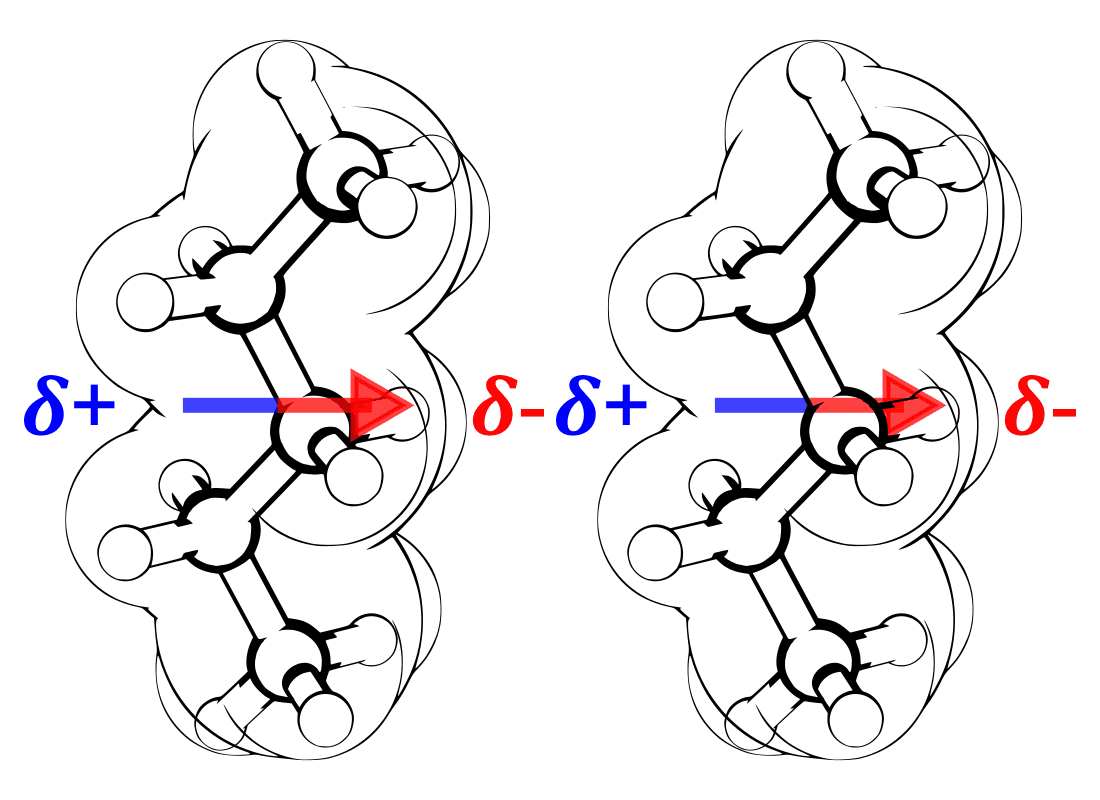
Figure 6. LDFs as molecular dipoles.
Each assertion in the following list is false:
- Misconception 1. Intermolecular Forces (IMFs) result from single, monolithic interactions between pairs of molecules.
Based on my interactions with teachers, this is the single most pervasive misunderstanding about IMFs, including LDFs.
Many teachers seem to think that because they are called intermolecular forces, they must involve only interactions at the molecule-molecule level.
Of the three most important IMFs (dipole-dipole, hydrogen bonds, and LDFs), only dipole-dipole interactions involve a single interaction between any pair of molecules. Hydrogen bonding and LDFs do not work this way.
If this misconception applies to you, and you change only one thing about how you teach IMFs – fix this one.
- Misconception 2. LDFs Involve Single, Temporary Dipole Moments that Span Whole Molecules.
This is a specific instance of misconception #1, above.
Take a close look at Figs. 5 and 6, above:
Fig. 5 (left) represents how LDFs in molecules actually work, and are simulated in Atomsmith.
Fig. 6 (right) is how LDFs are commonly taught.
Note: If the remainder of this section doesn’t convince you, perhaps this will:
We already have a type of IMF that involves single interactions between whole-molecule dipoles.They are called dipole-dipole forces. We don’t need another.
How was it decided to use molecular dipoles instead of atomic dipoles to explain LDFs?
I’m not sure, but I hypothesize that many textbook authors started with noble gas LDFs and naively extended the idea to molecules. This sort of works for only the smallest of molecules (2 - 3 atoms). But there’s no reason to apply this reasoning, not even for small molecules.
And then, my guess is that momentum took over. Textbook authors read others’ textbooks. But – apparently – they have not read the IMF theory and simulation literature.
As (hopefully) I have demonstrated, the simulation community has used atom-atom interactions to model LDFs since the early 1960s. And, we have known about this for far longer. In fact, Fritz London wrote about it in 1936.
He even called it “obvious”:

Figure 7. Fritz London called it “obvious” that LDFs in molecules should be treated at the level of atom-atom interactions – not molecule-molecule interactions. Notice that London used similar phrasing to Stone’s in Fig. 3 (“For all but the smallest molecules…”). (London1936)
I believe that Fritz would be a bit surprised at how we teach the concept that he first taught us almost a century ago.
None of this would matter, so much, if there were not actual consequences.
The biggest conceptual consequence of the LDF misconceptions is that, by definition, they can be only INTER-molecular. This ultimately leads to the problem of proteins not folding – which is where I started this essay.
Closer to home – in chemical education – there are also consequences for that most fundamental property that we depend on LDFs to teach: the ordering of boiling points in nonpolar molecules.
What is the classic pair of molecules used to demonstrate how LDFs determine alkane boiling points?
n-pentane (extended shape) and neopentane (compact shape)
They are an obvious example because, although they are different structural isomers of pentane, n-pentane is a liquid at room temperature and neopentane is a gas.
Here’s how one of the most popular (according to Google) websites about polarizabiliity and LDFs explains this phenomenon:

Figure 8. (Source)
In this narrative, polarizability refers to molecular polarizability – not atomic polarizability.
This sentence deserves special attention:
“Elongated molecules have electrons that are easily moved increasing their polarizability…”
In other words, long alkanes (only the long ones) behave as some kind of strange semiconductor: when they get close to each other, their atoms become like metals and their electrons freely flow between them.
This is incorrect.
The specific claim – that because neopentane is more compact, it is less polarizable, and therefore its (molecular-dipole-based) LDFs interactions are weaker, making it a gas, and that n-pentane exhibits greater molecular polarizability, so it is a liquid, is false
Variations of this explanation can readily also be found in many textbooks.
Momentum…
Molecular polarizabilities (αmol) are a property that you can actually look up:
molecule αmol (Å3) neopentane (gas) 10.24 n-pentane (liquid) 9.879 Yes, you read that correctly: neopentane has a higher molecular polarizability than that of n-pentane.
So, by the logic of how we teach LDFs, neopentane should be the liquid and n-pentane should be the gas.
…Consequences
In the same source as Fig. 8, there is an exhaustive discussion about how polarization of electrons occurs due to a uniform electric field caused by two charged plates. (Fig 9.). Uniform implies that the field’s magnitude is consistent across the entire sample.

Figure 9. Electron polarization in a uniform electric field. (Source)
Uniform electric fields have nothing to do with the LDFs in actual substances. I’ll bet that you will never boil a sample of n-pentane between two charged plates.
What is the real nature of the electric fields that atoms in molecules experience? They are from tiny, temporary atomic dipoles that are so small that the atoms must be very close to each other to have any effect.
Remember the $r^{-6}$ dependence of the attractive term in the Lennard-Jones potential?
Here’s what that means. If you double the distance between any two atoms that interact via their atomic dipoles, the LDF interaction energy at the new distance will be $\frac {1}{64}$ of the original energy ($\times 2^{-6}$).
And the LDF force between the atoms will be $\frac {1}{128}$ of the original force, because the force varies as $r^{-7}$.
Consider the distances between two pairs of hydrogen atoms in two neopentane molecules (Fig. 10, below). The LDF interaction energy between atoms H1 and H2 is about 0.1 kJ/mol.
The H2-H3 distance is a little more than double that of H1-H2. Therefore its LDF energy is less than 0.0016 kJ/mol. That’s why there is no thin blue line between those two atoms – the LDF interaction between them is negligible.

Figure 10. Distances of hydrogen atom - hydrogen atom LDF interactions in neopentane:
H1-H2: 3.13 Å
H2-H3: 6.90 ÅThe tiny electric fields produced by the atomic dipoles are too small to reach across most molecules. Go back and look at the n-pentane molecules in Fig. 5 (How LDFs Really Work). Notice that the left-most and right-most atomic dipoles are not aligned because they’re too far apart.
In Fig. 6 (How LDFs are Taught), the dipole spans the whole molecule and there is an indication of a partial postive charge (𝜹+) to the left and a partial negative charge (𝜹-) to the right. This is what you would expect if the molecules were sitting between charged plates – in a uniform electric field.
It just doesn’t work like that.
- Misconception 3. We cannot really “rank” the strengths of the different IMFs.
Here’s a common scenario. A teacher asks:
“I was taught that LDFs are the weakest IMF. But I was also taught that LDF energy can have a really large effect. What‘s up with that?”
A commonly offered response: “It’s not possible to order the strengths of IMFs. So you can’t really say that LDFs are the weakest IMF.”
The correct answer: LDFs are the weakest IMF – by far. But that’s in the context of individual atom-atom interactions – which is what was meant when you first learned about them.
Moving up the energy ladder: next come dipole-dipole interactions; then hydrogen bonds. (And yes, of course there are exceptions. This is chemistry.)
- Misconception 4. LDF energy correlates with molar mass.
If you tell your students this, the attentive ones who have already studied physics are gonna wanna apply this equation to LDFs: $${F_{g}}=G \frac {m_{1}m_{2}} {r}$$
And they would not be unjustified.
- Misconception 5. LDFs correlate with the total number of electrons.
Remember that atomic dipoles depend on atomic polarizabilities (~atomic volume) and numbers of valence electrons. The core electrons are not very polarizable.
Also remember that neopentane and n-pentane have the same number of electrons, yet one is a gas and one is a liquid. Clearly the total number of electrons cannot explain this fact. (We have already covered the fact that molecular polarizability also cannot explain this.)
- Misconception 6. LDFs correlate with a molecule’s surface area.
This one isn’t actually all that bad. It means that the more the surfaces of two molecules come in contact, the more LDF energy stabilization will occur.
Now that you understand how LDFs really work, here’s a much better way to say that:
Molecular shapes that result in more atom-atom interactions result in more LDF stabilization.
This statement is simple, and it is universally true, and applies to both intramolecular and intermolecular LDFs.
- Misconception 7. The name “dispersion force” refers to the electrons that are distributed (or dispersed) in the electron cloud […] or some other quantity that is “dispersed”.
London’s decision to name them “dispersion forces” has nothing to do with the “dispersal” of anything. Rather, it is due to his recognition that, some of the equations in his derivation of the $C_6$ constant are the same as those found in the theory of the dispersion of light, which describes the dependence of the index of refraction on the frequency of the radiation (Truhlar2019).
- Misconception 8. There is no such thing as INTRA-molecular LDFs.
I know. I beat this one to death with proteins. But I wanted to show the following cool pictures.

Figure 11. C200H402 with only INTER-molecular LDFs displayed. (There are none.)

Figure 12. C200H402 with INTRA-molecular LDFs displayed.
The plastic jugs that you use to carry home your milk from the market are made from high density polyetheylene (HDPE). “High density” means that some of the polymer is crystalline.
The long polyethylene chains fold back on themselves to form “crystallites”, which imparts enormous toughness to HDPE materials. These crystalline regions are made possible due to intra-molecular LDFs.
Fig. 11 displays all of the INTER-molecular LDFs in the (C200H402, standing in for polyethylene) crystal – all 0 of them.
Fig. 12 displays all of the INTRA-molecular LDFs in the crystal – all 177,309 of them.
So, there most certainly are INTRA-molecular LDFs after all.

Figure 13. Individual LDF interactions may be weak, but there is strength in numbers! (Source)
All Out of Bullets
If you are not yet convinced of the many flaws in the ways that we commonly teach LDFs, consider the following.

Figure 14. C6H12: 3-hexene and cyclohexane
A common follow-up exercise to the (incorrect, with respect to molecular polarizabilities) explanation of the neopentane and n-pentane boiling points is to challenge students to predict the relative boiling points of 3-hexene and cyclohexane (both C6H12).
Presumably the intent is to encourage students to recognize that the molecules are isomers, but that their shapes are different – in the same pattern as n-pentane and neopentane.
molecule formula molar mass (g/mol) total electrons (assumed) shape surface area (Å2) αmol (Å3) boiling point (°C) 3-hexene C6H12 84.16 48 extended 628 11.65 66 cyclohexane C6H12 84.16 48 compact 568 11.0 80.75 As I have discussed, in the table above, the molecular properties in columns 3 (molar mass) through 7 (molecular polarizability) are commonly used to predict the boiling points in column 8.
Is there any teacher who has assigned this exercise and is not surprised to see the actual boiling points in column 8? (I assume that no one assigns this exercise in order to trick their students.)
Is there a molecular or atomic property that can correctly correlate the LDFs and boiling points of 3-hexene and cyclohexane?
Yes!
In the liquid state, the number of atom-atom contacts between the cyclohexane molecules is greater than the number of atom-atom contacts between the 3-hexene molecules.
It’s really as simple as that. That’s the best we can do and that’s OK.
Finally, the data in the table above tell us something: the actual 3D shape of 3-hexene is not just its most extended form, as we may imagine it. As you can see below, there are many different shapes of 3-hexene:

Figure 15. Shapes of 3-hexene isomers. (vanHemelrijk1981)
LDFs in Action!
In Animation 3, below, you can see a simulation in Atomsmith’s Live Lab of the LDF interactions in liquid CCl4 (at a temperature below its boiling point).
If you are already a subscriber, and want to see what happens when you raise the temperature above the boiling point of CCl4, you can perform this simulation by opening the Experiment titled, “LDF (3) London Dispersion Forces in Action” in the Intermolecular Forces & States of Matter section of the Experiments menu.
If you are not a subscriber and you want to try out Atomsmith’s models so that you and your students can experience LDFs in action, just request a trial license here:
Notes and References
- C.N. Pace, et al (2014). Forces Stabilizing Proteins. FEBS Lett. 2014 June 27; 588(14): 2177–2184.
- R. Clausius (1857). XI. On the nature of the motion which we call heat. Philosophical Magazine Series 4, 14:91, 108-127.
The first known contemplation of attractive interactions between molecules in the condensed states dates to Clausius in 1857, as he considered differences between the liquid and the gaseous state:

- Silva, A.F., et al. (2020) Contributions of IQA electron correlation in understanding the chemical bond and non-covalent interactions. Struct Chem 31, 507–519.
- Pauli Repulsion. The repulsion that occurs between atoms at close distances is due to a quantum mechanical effect called Pauli Repulsion (aka Exchange Interaction). This is related to the Pauli Exclusion principle, in which no two electrons can occupy the same state – which they would when the atoms get too close to each other.
- London, F. (1930). Zur Theorie und Systematik der Molekularkräfte. Zeitschrift für Physik, 63 (3–4): 245.
- London, F. (1936). The general theory of molecular forces. Transactions of the Faraday Society, 33, 8b.
- B.J. Alder, T.E. Wainwright (1958). Molecular Dynamics by Electronic Computers, in I. Prigogine (ed.), Proceedings of the International Symposium on Transport Processes in Statistical Mechanics (Brussels, August 27–31, 1956), Interscience Pub., London, pp. 97–131.
- Rahman, A. (1964). Correlations in the Motion of Atoms in Liquid Argon. Physical Review, 136(2A), A405–A411.
- McCammon JA, Gelin BR, and Karplus M (1977). Dynamics of Folded Proteins. Nature 267, 585–590.
- Stone, A. J. (2013). The Theory of Intermolecular Forces. Oxford: Oxford University Press.
- Truhlar, D. G. (2019). Dispersion Forces: Neither Fluctuating Nor Dispersing. J. Chem. Educ. 96, 1671−1675.
- Van Hemelrijk, D., van den Enden, L., & Geise, H. J. (1981). The molecular structures of cis-3-hexene and trans-3-hexene in the gas phase by electron diffraction and molecular mechanical calculations. Journal of Molecular Structure, 74(1), 123–135.